A Vacuum System Consolidation Audit

Vacuum systems are considered “black magic” by most plant engineers, even more so than compressed air. Terms like icfm, cfm, torr, and Nm3/hr get bandied around and confuse us all. What plant engineers know is what works. If they run vacuum pump X at vacuum level Y, everything works. That is a hard thing to change if there are inefficiencies in the system, even when an audit is recommending change. One of the biggest opportunities I run into for savings is the consolidation of multiple vacuum systems running at a lower absolute pressure (higher vacuum) than is really needed. Therefore, educating the customer is critical.

 

Vacuum System Basics

Before I launch into the actual audit, let me define a couple of key terms relating to vacuum systems:

Capacity: As with compressors, this is the inlet flow volume that the vacuum pump pulls in at a given vacuum and speed. For positive-displacement vacuum pumps, which are evaluated in this audit, capacity is fairly constant (at constant speed). It is measured in ft3/min, and called icfm in Imperial units, and m3/hr in SI units.

Vacuum: This is the gauge pressure that the inlet is at, relative to the atmospheric pressure. Usually this is in inches of Mercury (0” Hg) in Imperial and mbar or torr in SI units.

Free Airflow: This term is used less often, but is critical to understanding consolidation. This is the air, in scfm (Imperial) or Nm3/hr (SI), that the process pulls into the system—if it is at sea level. Free airflow is directly proportional to inlet absolute pressure, assuming a constant capacity. In other words, at 20” Hg vacuum (about 10” Hg absolute pressure), the vacuum pump’s free air delivery will be at 33 percent of its capacity. At 22” Hg vacuum (20” absolute), it will be at 26.7 percent. The change in capacity from 22” to 20” Hg is 26.7/33.3 = 0.80, a 20 percent decrease in required capacity.

System Curve: The process is merely an orifice, with atmospheric pressure on the front end and vacuum on the other. Like an orifice, the relationship between vacuum and flow that the system requires is “second order.” That is, vacuum is proportional to the square root of flow, and flow is proportional to the square root of vacuum. Thus, lower vacuum will require less flow in scfm. Running at 20” Hg instead of 22” Hg will require (20/22)0.5 = 0.95, or about 5 percent less delivered air.

Thus, reducing vacuum reduces the required capacity in two ways. First, it reduces the free air (by the square root of the vacuum ratio). Secondly, there is less capacity required to deliver that reduced free air (linearly by the ratio of the absolute pressure). Changing vacuum level from 22” Hg to 20” Hg can drop the required capacity by about 24 percent (1.0 - 0.80 x 0.95). If one was to consolidate a system of four vacuum pumps with that drop in vacuum, one vacuum pump could be shut off for a majority of the time. That is the basis for the consolidation savings in this proposed project.

 

Initial Vacuum System Description

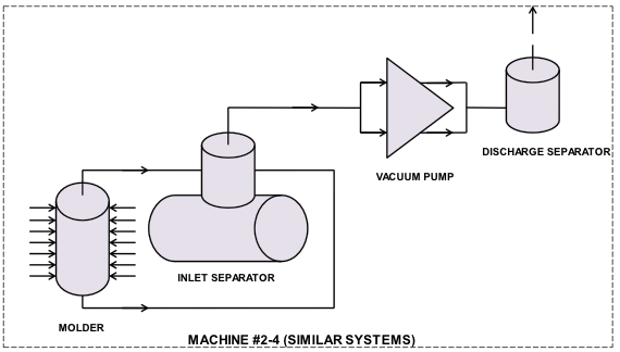
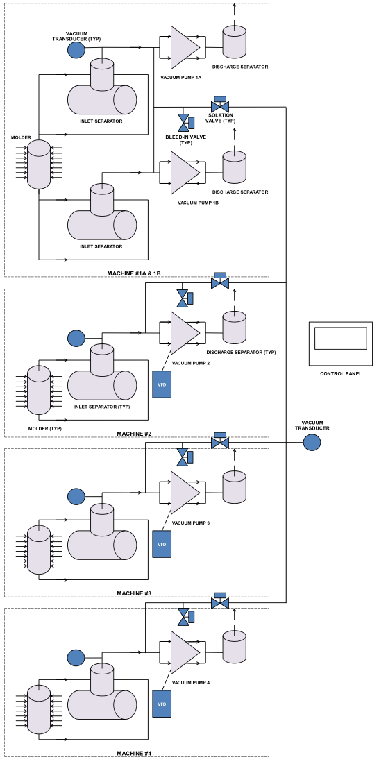
Refer to Figures 1 and 2 for simplified diagrams of the four systems. Three are identical 200-hp, 4000 acfm, liquid-ring vacuum pump systems, supplying machines two through four. They currently run continuously at 23” Hg, except during brief shutdowns. Machine One is a smaller, 75-hp duplex system, approximately 2300 acfm. It runs about 25 percent of the time for special orders, at about 20” Hg. Total system demand is 10,000 icfm at 21” Hg, or about 2450 scfm.

 

Figure 1: Vacuum Piping Schematic for Machine One (A & B)

 

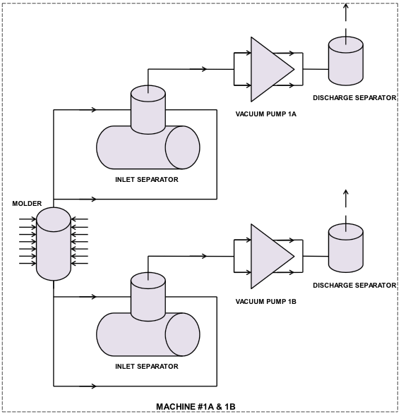
Figure 2: Existing Vacuum Piping Schematic for Machines Two Through Four

 

Energy Efficiency Measures

Three multiple, mutually exclusive options for energy efficiency improvements have been considered for the vacuum system. These options were developed to provide alternatives if the theoretical customer, let’s say Customer ABC, has limited funding. In our view, Measure 1A is superior.

Measure 1A: Integrate the Vacuum Systems

Currently, the four systems (Machines One through Four) run separately. The vacuum level is uncontrolled, seeking its own on the vacuum pump curve at a level in excess of what is needed. The combined flow demand from all lines can be significantly dropped if vacuum is dropped. However, when operating separately, the individual vacuum pumps can’t be turned down enough to match the reduction opportunity possible through vacuum set point reduction. With the connecting pipe, the vacuum pumps can be optimally controlled at the reduced vacuum/flow. A large vacuum pump can be shut off most of the time if an automation system can manage the vacuum pumps.

This project includes piping, variable frequency drives (VFDs) and controls to optimally run the system at one common vacuum level. Flexibility is built into the recommended system design to allow for segmentation of the system, if future products would require different vacuum levels. Energy efficiency will not be compromised if that occurs.

Measure 1A offers the most flexibility and savings. The system can be run at the same vacuum level or at multiple levels. It can meet very high and very low demands, while still maintaining efficiency. Additionally, one or more vacuum pumps will be off most of the time to accommodate maintenance or standby.

Measure 1B: Install VFDs on Individual Vacuum Pumps

This is a lower-cost alternative to Measure 1A. This measure adds VFDs to each 200-hp vacuum pump (Machines Two through Four), keeping them separate. It has some of the flexibility of Measure 1A, but it does not yield as much savings.

Measure 1C: Change V-Drive Speeds of Each Vacuum Pump

This measure consists of changing sheaves and possibly belts, so that each vacuum pump operates at the target vacuum level. Just the three larger units (Machines Two through Four) would be changed.

 

Economic Summary

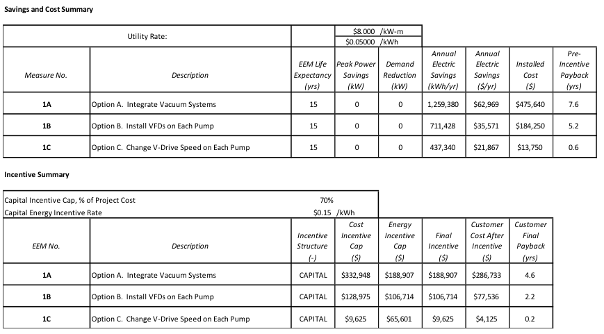
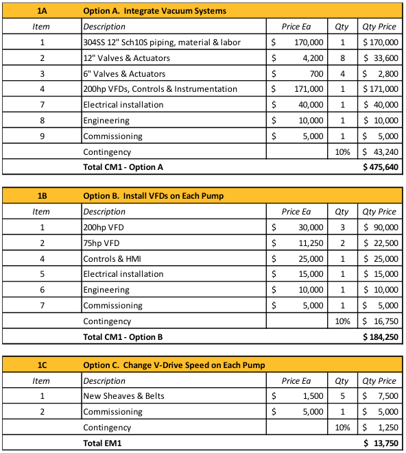
Table 1 provides a summary of the estimated costs, benefits and potential incentives for the custom energy efficiency measures evaluated in this report. The potential utility incentives for capital-intensive, custom measures are calculated as $0.15 times the total project energy savings (in kWh), subject to project-level caps. The incentive shall not exceed 70 percent of the eligible project cost or the amount that results in a one-year payback based on energy cost savings.

 

Table 1: Cost, Savings and Incentives Summary

Click here to enlarge

 

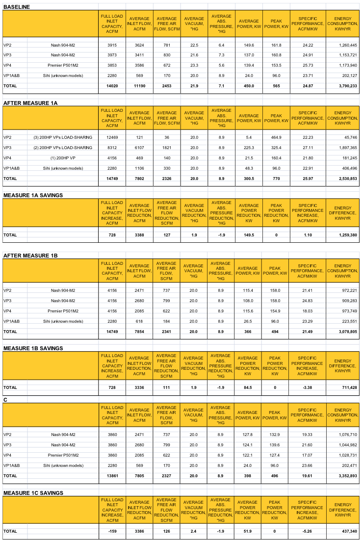
The optional measures reduce system energy use by 19 to 33 percent, depending on the option selected, and produce a simple payback of 0.2 to 4.6 years after the potential utility incentive.

Electrical savings are much higher if the vacuum system can be run at a lower level. For instance, at 17” Hg, savings from Measure 1A are over 2,050,000 kWh/yr, yielding a project payback of less than 2 years. An initial test was successfully run at 17” Hg on Machine Two. However, subsequent testing showed that additional gas usage in the dryer would be needed for vacuum levels lower than about 20” Hg, which would have been “fuel switching.” This type of trade-off was not cost-effective, and would disqualify the project from potential utility incentives.

However, if Customer ABC could run the system at lower than 20” Hg without additional gas, the savings would be approximately 320,000 kWh/yr more for each 1.0” Hg lower than 20” Hg, down to 18” Hg, and 240,000 kWh/yr more to get to 17” Hg. The incentive would increase by $0.15/kWh for Measure 1A ($48,000) per every 1” Hg down to 18” Hg. For this reason, and the additional reliability, flexibility and controllability provided by Measure 1A, we would recommend this measure if Customer ABC had enough capital.

 

Detailed Description of Proposed Equipment and Operation

Measure 1A: Integrate Vacuum Systems

Source of Energy Savings

The measure combines the four systems, controls the number of vacuum pumps running, and runs them at their most efficient speed. This saves energy in four ways:

1. Operating a vacuum system at a lower vacuum (higher absolute pressure) significantly reduces the excess flow requirement at the vacuum pump inlet to achieve a given mass flow requirement. If a system can operate at 20” Hg (9” Hg absolute in Yakima, WA), and operates at 23” Hg (6” Hg absolute), it requires 9/6 the acfm volume to develop the same scfm real-system demand.
2. Operating at a deeper vacuum than needed also requires more mass flow of air than needed— about 7 percent more in the above example.
3. These vacuum pumps are more efficient at lower speed, likely due to less hydraulic losses.
4. Running fewer vacuum pumps in a combined system allows the speed optimization to occur. Instead of running pumps at maximum speed or at minimum speed with too much capacity for the demand, the right number of pumps as a set will be running.

Specific Equipment Recommendations

Refer to Figure 3 for a system sketch:

Install VFDs on the three 200-hp vacuum pumps (Machines Two through Four).

• Install vacuum transducers at each of the four inlet separators.
• Install a 12” stainless steel header, with four branch lines to connect the inlets of all four systems to the header. The branch lines are on the vacuum pump side of the vacuum-regulating valves.
• Install four 12” automatic butterfly valves on the individual branch lines for isolation from the header, normally open.
• Install four 6” automatic butterfly valves at the vacuum pump inlets, on tees to atmosphere, for unloaded starting and testing, normally closed.
• Install a master control system to control the following:
  • Vacuum level at each machine, and vacuum at the main header.
  • Vacuum pump speed.
  • Vacuum pump start and stop, based on a flow-based algorithm, running exactly the right combination of vacuum pumps in every flow range. This controls vacuum at the header.
  • Isolation butterfly valve operation.
  • Bleed-in valve operation.
• Interface the controls with the plant supervisory control and data acquisition (SCADA) system and/or PI system for data collection and trending.
• Preliminary staging is shown in Table 2.

 

Table 2: Vacuum Pump Staging

“T” = “trim,” or party-loaded

“B” = base-load, or fully loaded

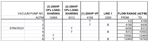
Figure 3: Recommended System Diagram for Measure 1A

Performance Indicators Recommended to Achieve Optimal Energy Efficiency

• Target a common vacuum of 20” Hg to start. Lower vacuum creates more savings. However, we don’t recommend going much lower due to the need to add more natural gas in the drying section.
• Run the vacuum pumps in a “load-sharing” algorithm, running multiple units at as low a speed as possible. The minimum speed is 300 rpm, which is about 85.7 percent of full speed.

Additional Assumptions Behind the Savings Estimate

• The vacuum pumps operate according to the manufacturer’s pump curve.
• The VFD’s efficiency is 97 percent.
• Motor efficiency is constant throughout the operating range of the VFD.
• Pipe length and elevations used in analysis are accurate estimates.

 

Measure 1B: Install VFDs on Individual Vacuum Pumps

Source of Energy Savings

The sources of savings are the same as the first three for Measure 1A. Savings are less because a vacuum pump can’t be completely shut down until the line goes down.

Specific Equipment Recommendations

• Install VFDs on the three 200-hp vacuum pumps (Machines Two through Four) and the two 75-hp vacuum pumps (Machine One, A & B).
• Install vacuum transducers at each of the four inlet separators.
• Install controls at each line to control the following:
  • Vacuum level
  • Vacuum pump speed
• Interface the controls with the plant SCADA and/or PI system for data collection and trending.

Performance Indicators Recommended to Achieve Optimal Energy Efficiency

• Target a vacuum of 20” Hg to start. Lower vacuum creates more savings. However, we don’t recommend going much lower due to the need to add more natural gas in the drying section.
• The minimum speed is 300 rpm, or 85.7 percent of full speed.

Additional Assumptions Behind the Savings Estimate

• The vacuum pumps operate according to the manufacturer’s pump curve.
• The VFD’s efficiency is 97 percent.
• Motor efficiency is constant throughout the operating range of the VFD.

 

Measure 1C: Change V-Drive Speeds of Each Vacuum Pump

Source of Energy Savings

The sources of savings are the same as numbers one through three, as outlined in Measure 1A, but at a lower level.

Specific Equipment Recommendations

• Change the V-belts and sheaves of each of the vacuum pumps so that they can operate at about 21” Hg at full production. This gives some additional head room since there is no drive to increase speed. The preliminary speeds are as follows:
  • Machine Two: 338 rpm
  • Machine Three: 344 rpm
  • Machine Four: 331 rpm

Performance Indicators Recommended to Achieve Optimal Energy Efficiency

• Target a vacuum of 21” Hg to start. Lower vacuum creates more savings.
• The minimum speed is 300 rpm, or 85.7 percent of full speed.

Additional Assumptions Behind the Savings Estimate

• Same as Measure 1B, except for VFD losses

 

Modeling Results                                                                 Click here to enlarge

 

Cost Estimates

 

For more information, contact Tim Dugan, P.E., President, Compression Engineering Corporation by phone at (503) 520-0700, or visit www.comp-eng.com.

To read similar articles about Vacuum System Assessments, please visit www.blowervacuumbestpractices.com/system-assessments.

 

---