Sizing, selection, and adjusting control valves often causes confusion for process and control system designers. Improper valve application can cause operating problems for plant staff and waste blower power. Basing the airflow control system design on fundamental principles will improve valve and control system performance.
The Law of Conservation of Energy and the Law of Conservation of Mass govern the behavior of control valves. When a concept or a conclusion seems questionable, or unfamiliar technology is being examined, these two fundamental principles must form the basis of the evaluation.
In this first of a two-part article, we will examine valve operating and analysis basics.
Creating Pressure Differential
The function of any valve is to create a pressure differential between the upstream and downstream piping. If the valve is employed as a shut-off device the differential is equal to the full upstream pressure. In aeration applications, valves are also used to create the pressure differential required to control airflow rates – a process known as throttling.
The pressure differential across a valve is dependent on many factors. Fluid properties are significant but are generally outside the control of the system designer. The mechanical design of the valve and the nominal diameter are also important, and they are amenable to designer selection. In most aeration applications butterfly valves (BFVs) are used for control, but alternate designs are available.
Regardless of the type of valve, or its size, the restriction to flow can be quantified by the flow coefficient, Cv. This is defined as the gallons per minute of water flowing through a valve with a pressure differential of 1.0 psi. The greater the flow coefficient the lower the restriction to flow the valve creates. The coefficient increases as valve diameter increases, or as a given valve moves open. Most valve suppliers publish the Cv data for various diameters and positions as shown in Figure 1 and Figure 2.
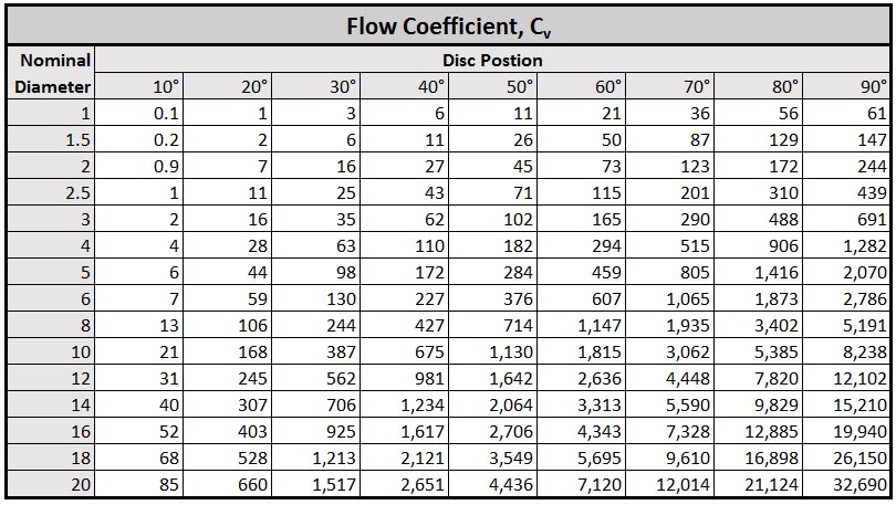
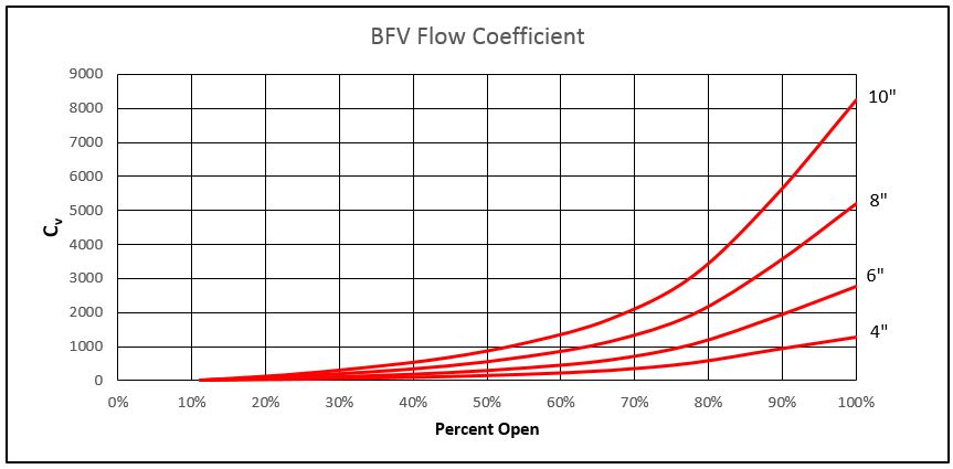
Shown in Figure 1 is an example of tabulated flow coefficient data for a butterfly valve. Figure 2 is an example of graphical flow coefficient data for a butterfly valve.
If the conditions of flow are known the airflow rate for a given Cv can be calculated:
Where:
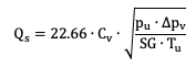
Qs = airflow rate, SCFM
Cv = valve flow coefficient from manufacturer’s data, dimensionless
pu = upstream absolute air pressure, psia
Δpv = pressure drop (differential) across the valve, psi
SG = specific gravity, dimensionless, = 1.0 for air
Tu = upstream absolute air temperature, °R
In ISO units, the flow coefficient is expressed as Kv. This is defined as the flow in cubic meters per hour of water at a pressure differential of 1 bar.
![]()
It is often necessary to determine the pressure drop for a known flow coefficient, or to determine the flow coefficient corresponding to a known pressure drop and flow:
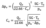
These relationships are non-linear. The variation in Cv with position is also nonlinear for most types of valves. This non-linearity may create problems with control precision if the design or controls aren’t appropriate.
There are many assumptions inherent in any set of fluid flow calculations. Accuracy better than plus or minus 10% should not be expected. This accuracy is adequate for most systems. Margins of safety and adjustment capabilities should be used in the design to accommodate uncertainties.
Bernoulli’s Law in Airflow Control Analysis
In airflow control analysis, Bernoulli’s Law is important. It shows that the total energy in the air stream on both sides of a valve is identical. This is an extension of the Law of Conservation of Energy. The energy in the moving air consists of three components, as show in Bernoulli’s Law:
![]()
Where:
p1,2 = potential energy = static pressure, psi
ρ = density at airflow conditions, lbm/ft3
V1,2 = air velocity, ft/min
Δpf = pressure drop due to friction, psi
Velocity can be readily calculated based on the Law of Conservation of Mass:
![]()
The Law of Conservation of Mass shows that on both sides of a valve the velocity is equal unless pipe diameter changes:
![]()
Where:
Qa = volumetric flow rate at actual conditions, ACFM (actual ft3/min)
A1,2 = cross sectional area of pipe, ft2
V1,2 = velocity, ft/min
The velocity term in Bernoulli’s Law represents the kinetic energy of the airflow. It is called dynamic pressure (pd), velocity pressure, or velocity head. In most aeration systems the dynamic pressure is negligible compared to the static pressure as depicted in Figure 3. Furthermore, unless there is a change in pipe diameter or a significant change in air density the velocity and dynamic pressure upstream and downstream of the valve are basically equal, regardless of valve type.
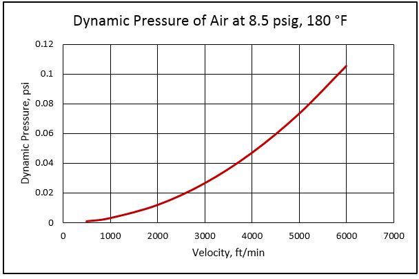
Figure 3: Dynamic pressure (velocity head) for a typical aeration application.
The blower system must create the total pressure needed to move air through the piping system and diffusers. The largest component of system pressure results from diffuser submergence. This static pressure is 80 to 90 percent of the total pressure in most aeration systems and is essentially constant.
Valve pressure drop is typically the next largest component of blower discharge pressure. Pressure drops through a BFV or other valve represent a parasitic loss. The frictional energy from the pressure drop across the valve is converted to heat. In a typical aeration system the valves share a common distribution header with uniform upstream pressure. The downstream pressure is nearly identical at all valves because diffuser submergence is identical. Therefore, the value of Δpf is virtually the same for all valves in a system.
The pressure drop through a valve is used to modulate flow to individual process zones. The valve is adjusted until the airflow through the valve equals the process demand. The pressure differential equals the available difference between upstream and downstream pressures.
In any system there is pressure drop through distribution piping upstream of the valve and through the piping and diffusers downstream of the valve. These losses are generally a small part of the total pressure requirement. In real systems the diffuser pressure drop and piping losses may not be negligible. However, diffuser and piping losses, like valve throttling, are a function of airflow rate. Differences from tank to tank simply reduce the amount of throttling required from the valve.
Frictional pressure drops do increase the blower discharge pressure and therefore blower power demand. Energy optimization includes minimizing valve losses. Minimizing energy with low valve losses must be balanced against the need to create pressure losses in order to control flow. These conflicting needs can make proper valve sizing a challenge. Minimizing frictional pressure drop while maintaining controllability necessitates the need to use realistic air velocities for design as outlined in Figure 4.
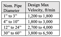
Figure 4: Typical design velocity limits for aeration piping.
Control Valve Characteristics
The characteristics of control valves can be illustrated by examining a simple system with one valve, as shown in Figure 5. The system characteristics are the same regardless of control valve type. For illustrative purposes the pressure drops through the piping and aeration diffusers will be ignored.
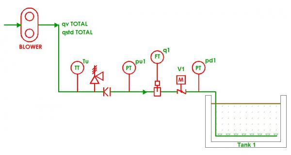
Figure 5: Shown is a simple blower system with one valve.
The pressure downstream of the valve, pd1, is established by assuming diffuser submergence of 19 feet, 7 inches, equal to 8.5 psig. Air temperature T1 is 640 °R (180 °F). Pipe diameter is 8 inches nominal Schedule 10 pipe, and a BFV is used for throttling.
The system is analyzed across an airflow range of 250 SCFM to 1,500 SCFM (qstd TOTAL). That corresponds to volumetric flow rates downstream of the BFV between 190 ACFM and 1,100 ACFM (qv TOTAL) and a velocity range between 500 ft/min and 3,000 ft/min. These are within normal design limits for 8-inch pipe. The blower is assumed to be a positive displacement type, and at fixed speed the flow rate is constant regardless of discharge pressure.
When the valve is throttled the pressure differential obviously changes. What isn’t obvious from observing the equations is the loss of control at the upper and lower end of the BFV position range. At positions close to full open, the pressure drop changes very little as the valve closes. On the other end of the range, when the valve is nearly closed, very small position changes create dramatic changes in pressure drop as shown in Figure 6.
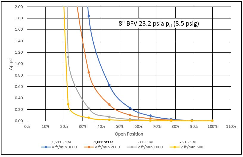
Figure 6: An example of Δp versus air velocity.
Two conclusions can be drawn from this. The first is that valve travel should be limited to the middle of the operating range. Control systems commonly limit travel to between 15 and 70 percent open. These values are not absolute, of course, and field experience on each system is needed to establish the most appropriate limits. Avoiding oversized valves and very low air velocities is important, since that keeps the valve opening within the controllable region.
The second conclusion is that it is necessary to have accurate control of position changes. Using actuators with slow operation is suggested, with 60 seconds or more per 90-degree rotation being common. Reducing the dead band and hysteresis on valve positioners to 1% or less also improves control.
Motor brakes on electric actuators improve accuracy. Many actuators have “self-locking” gears which prevent aerodynamic forces on the valve disc from back-driving and turning the stem when the motor is off. However, when the motor is powered to reposition the valve and then power is cut at the set position the motor will continue to spin, acting like a flywheel. This can drive the valve past the set position and induce errors and hunting. A brake on the motor engages as soon as power is cut and stops the valve at the set position.
Many blower control systems maintain a constant discharge pressure. In these systems the BFV position needed to regulate the basin airflow rate varies with the set discharge pressure and the corresponding Δp as depicted in Figure 7. Non-linearity is apparent in this diagram, but if both the pressure and travel ranges are kept within reasonable limits adequate control can be maintained. Note that absolute airflow rate precision is not needed for most aeration applications – slight errors will not materially affect process performance.
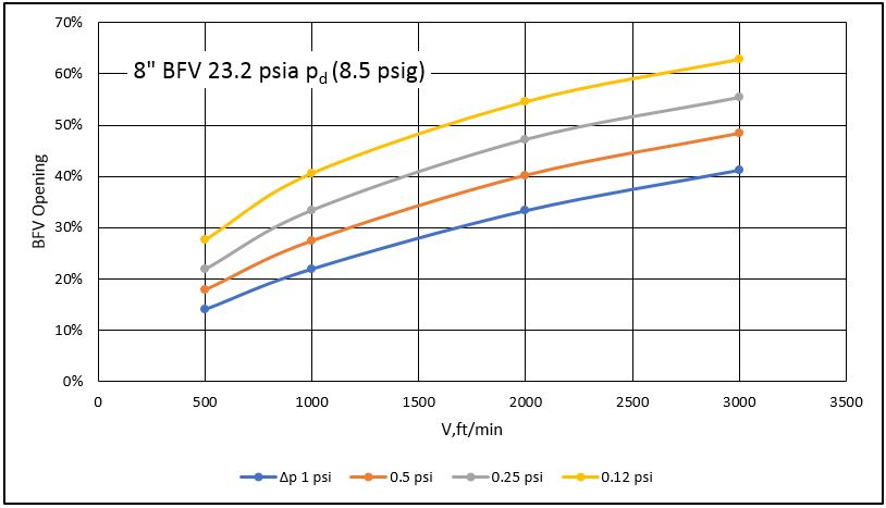
Figure 7: An example valve position to maintain constant Δp.
Conclusion
Valves must create pressure drops in order to control airflow by throttling. The relationship can be expressed mathematically using the valve’s Cv. For most valves the correlation between flow and pressure is nonlinear. Despite the nonlinearity, proper selection of size and actuator type will provide adequate control precision.
In the second article of this two-part series, we will examine the interaction of valves in parallel. New types of control valves and their performance will be compared to the baseline butterfly valve.
For more information contact Tom Jenkins, President, JenTech Inc., email: [email protected] or visit http://www.jentechinc.com/.
To read part 2 of these series, visit https://blowervacuumbestpractices.com/technology/aeration-blowers/basics-aeration-control-valves-%E2%80%93-part-2
To read similar articles on Aeration Blower Technology, please visit /technology/aeration-blowers.